Verilog Hacks
Because of the limited capability of FPGA computation, compromises often need to made in the actual Verilog implementation. The most used techniques include quantization and look up table. In OpenOFDM, these approximations are used.
Magnitude Estimation
- Module:
complex_to_mag.v - Input:
i (32), q (32) - Output:
mag (32)
In the sync_short module, we need to calculate the magnitude of the
prod_avg, whose real and imagine part are both 32-bits. To avoid 32-bit
multiplication, we use the Magnitude Estimator Trick from DSP Guru. In particular, the
magnitude of complex number \(\langle I, Q\rangle\) is estimated as:
And we set \(\alpha = 1\) and \(\beta = 0.25\) so that only simple bit-shift is needed.
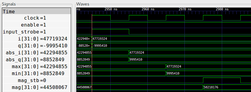
Fig. 27 Waveform of complex_to_mag Module
Fig. 27 shows the waveform of the complex_to_mag
module. In the first clock cycle, we calculate abs_i and abs_q. In the
second cycle, max and min are determined. In the final cycle, the
magnitude is calculated.
Phase Estimation
- Module:
phase.v - Input:
i (32), q (32) - Output:
phase (32) - Note: The returned phase is scaled up by 512 (i.e., \(int(\theta *512)\))
When correcting the frequency offset, we need to estimate the phase of a complex number. The right way of doing this is probably using the CORDIC algorithm. In OpenOFDM, we use look up table.
More specifically, we calculate the phase using the \(arctan\) function.
The overall steps are:
- Project the complex number to the \([0, \pi/4]\) range, so that the \(tan(\theta)\) range is \([0, 1]\).
- Calculate \(arctan\) (division required)
- Looking up the quantized \(arctan\) table
- Project the phase back to the \([-\pi, \pi)\) range
Here we use both quantization and look up table techniques.
Step 1 can be achieved by this transformation:
In the lookup table used in step 3, we use \(int(tan(\theta)*256)\) as the key, which effectively maps the \([0.0, 1.0]\) range of \(tan\) function to the integer range of \([0, 256]\). In other words, we quantize the \([0, \pi/4]\) quadrant into 256 slices.
This \(arctan\) look up table is generated using the
scripts/gen_atan_lut.py script. The core logic is as follows:
1 2 3 4 5 6 7 | SIZE = 2**8
SCALE = SIZE*2
data = []
for i in range(SIZE):
key = float(i)/SIZE
val = int(round(math.atan(key)*SCALE))
data.append(val)
|
Note that we also scale up the \(arctan\) values to distinguish adjacent
values. This also systematically scale up \(\pi\) in OpenOFDM. In fact,
\(\pi\) is defined as \(1608=int(\pi*512)\) in
verilog/common_params.v.
The generated lookup table is stored in the verilog/atan_lut.coe
file (see COE File Syntax).
Refer to this guide on
how to create a look up table in Xilinx ISE. The generated module is stored in
verilog/coregen/atan_lut.v.
Rotation
- Module:
/verilog/rotate.v - Input:
i (16), q (16), phase (32) - Output:
out_i (16), out_q (16) - Note: The input phase is assumed to be scaled up by 512.
To rotate a complex number \(C=I+jQ\) by \(\theta\) degree, we can multiply it by \(e^{j\theta}\), as shown in (4).
Again, this can be done using the CORDIC algorithm. But similar to Phase Estimation, we use the look up table.

Fig. 28 Quadrant in I/Q Plane
As shown in Fig. 28, we split the I/Q plane into 8 quadrants,
\(\pi/4\) each. To avoid storing nearly duplicate entries in the table, we
first map the phase to be rotated (\([-\pi, \pi]\)) into the \([0,
\pi/4]\) range. Next, since the incoming phase is scaled up by 512, each quadrant
is further split into \(402=int(\pi/4*512)\) sectors. And the
\(\cos(\theta)\) and \(\sin(\theta)\) values (scaled up by 2048) are
stored in the look up table. The table is generated by the
scripts/gen_rot_lut.py.