Packet Detection
802.11 OFDM packets start with a short PLCP Preamble sequence to help the receiver detect the beginning of the packet. The short preamble duration is 8 us. At 20 MSPS sampling rate, it contains 10 repeating sequence of 16 I/Q samples, or 160 samples in total. The short preamble also helps the receiver for coarse frequency offset correction , which will be discussed separately in Frequency Offset Correction.
Power Trigger
- Module:
power_trigger.v - Input:
sample_in(16B I + 16B Q),sample_in_strobe(1B) - Output:
trigger(1B) - Setting Registers:
SR_POWER_THRES,SR_POWER_WINDOW,SR_SKIP_SAMPLE.
The core idea of detecting the short preamble is to utilize its repeating nature by calculating the auto correlation metric. But before that, we need to make sure we are trying to detect short preamble from “meaningful” signals. One example of “un-meaningful” signal is constant power levels, whose auto correlation metric is also very high (nearly 1) but obviously does not represent packet beginning.
The first module in the pipeline is the power_trigger.v. It takes the I/Q
samples as input and asserts the trigger signal during a potential packet
activity. Optionally, it can be configured to skip the first certain number of
samples before detecting a power trigger. This is useful to skip the spurious
signals during the initial hardware stabilization phase.
The logic of the power_trigger module is quite simple: after skipping
certain number of initial samples, it waits for significant power increase and
triggers the trigger signal upon detection. The trigger signal is
asserted until the power level is smaller than a threshold for certain number of
continuous samples.
Short Preamble Detection
- Module:
sync_short.v - Input:
sample_in(16B I + 16B Q),sample_in_strobe(1B) - Output:
short_preamble_detected(1B) - Setting Registers:
SR_MIN_PLATEAU
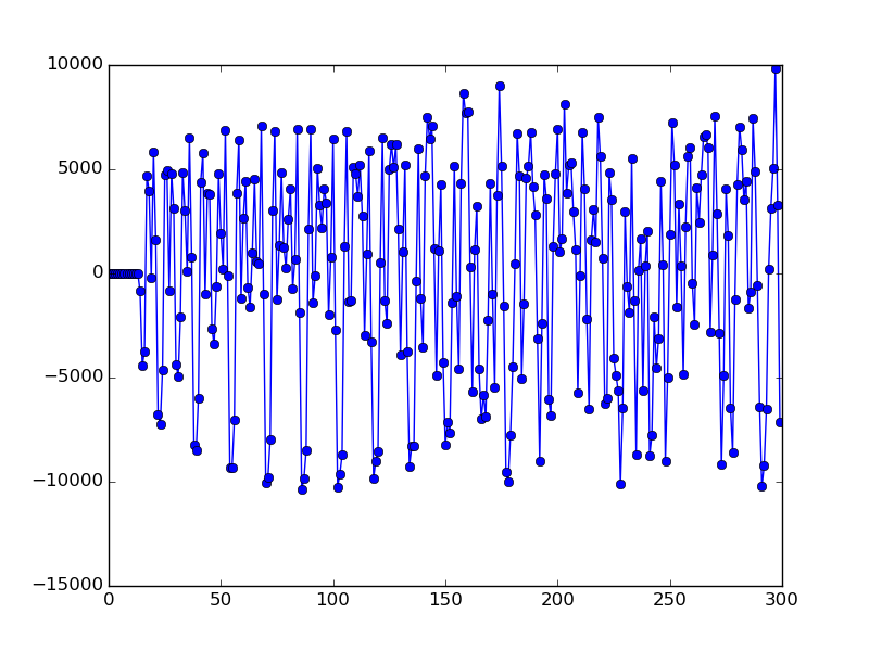
Fig. 2 In-Phase of Short Preamble.
Fig. 2 shows the in-phase of the beginning of a packet. Some repeating patterns can clearly be seen. We can utilize this characteristic and calculate the auto correlation metric of incoming signals to detect such pattern:
where \(S[i]\) is the \(\langle I,Q \rangle\) sample expressed as a complex number, and \(\overline{S[i]}\) is its conjugate, \(N\) is the correlation window size. The correlation reaches 1 if the incoming signal is repeating itself every 16 samples. If the correlation stays high for certain number of continuous samples, then a short preamble can be declared.
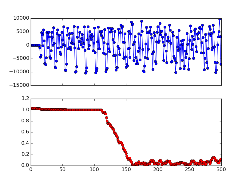
Fig. 3 Auto Correlation of the Short Preamble samples (N=48).
To plot Fig. 3, load the samples (see Sample File), then:
from matplotlib import pyplot as plt

fig, ax = plt.subplots(nrows=2, ncols=1, sharex=True)
ax[0].plot([s.real for s in samples[:500]], '-bo')
ax[1].plot([abs(sum([samples[i+j]*samples[i+j+16].conjugate()
    for j in range(0, 48)]))/
    sum([abs(samples[i+j])**2 for j in range(0, 48)])
    for i in range(0, 500)], '-ro')
plt.show()
Fig. 3 shows the auto correlation value of the samples in
Fig. 2. We can see that the correlation value is almost 1
during the short preamble period, but drops quickly after that. We can also see
that for the very first 20 samples or so, the correlation value is also very
high. This is because the silence also repeats itself (at arbitrary interval)!
That’s why we first use the power_trigger module to detect actual packet
activity and only perform short preamble detection on non-silent samples.
A straight forward implementation would require
both multiplication and division. However, on FPGAs devision consumes a lot of
resources so we really want to avoid it. In current implementation, we use a
fixed threshold (0.75) for the correlation so that we can use bit-shift to
achieve the purpose. In particular, we calculate numerator>>1 + numerator>>2
and compare that with the denominator. For the correlation window size, we set
\(N=16\).

Fig. 4 sync_short Module Diagram
Fig. 4 shows the internal module diagram of the sync_short
module. In addition to the number of consecutive samples with correlation
larger than 0.75, the sync_short module also checks if the incoming signal
has both positive (> 25%) and negative (> 25%) samples to further eliminate
false positives (e.g., when the incoming signals are constant non-zero values).
Again, the thresholds (25%) are chosen so that we can use only bit-shifts for
the calculation.