Sub-carrier Equalization and Pilot Correction
- Module:
equalizer.v - Input:
I (16), Q (16) - Output:
I (16), Q (16)
This is the first module in frequency domain. There are two main tasks: sub-carrier gain equalization and correcting residue phase offset using the pilot sub-carriers.
Sub-carrier Structure
The basic channel width in 802.11a/g/n is 20 MHz, which is further divided into 64 sub-carriers (0.3125 MHz each).
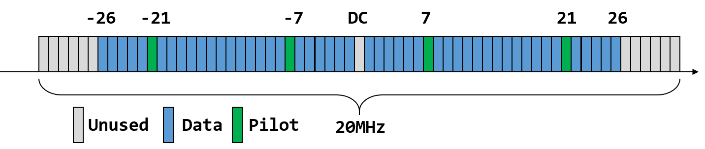
Fig. 13 Sub-carriers in 802.11 OFDM
Fig. 13 shows the sub-carrier structure of the 20 MHz band. 52 out of 64 sub-carriers are utilized, and 4 out of the 52 (-7, -21, 7, 21) sub-carriers are used as pilot sub-carrier and the remaining 48 sub-carriers carries data. As we will see later, the pilot sub-carriers can be used to correct the residue frequency offset.
Each sub-carrier carries I/Q modulated information, corresponding to the output
of 64 point FFT from sync_long.v module.
Sub-Carrier Equalization
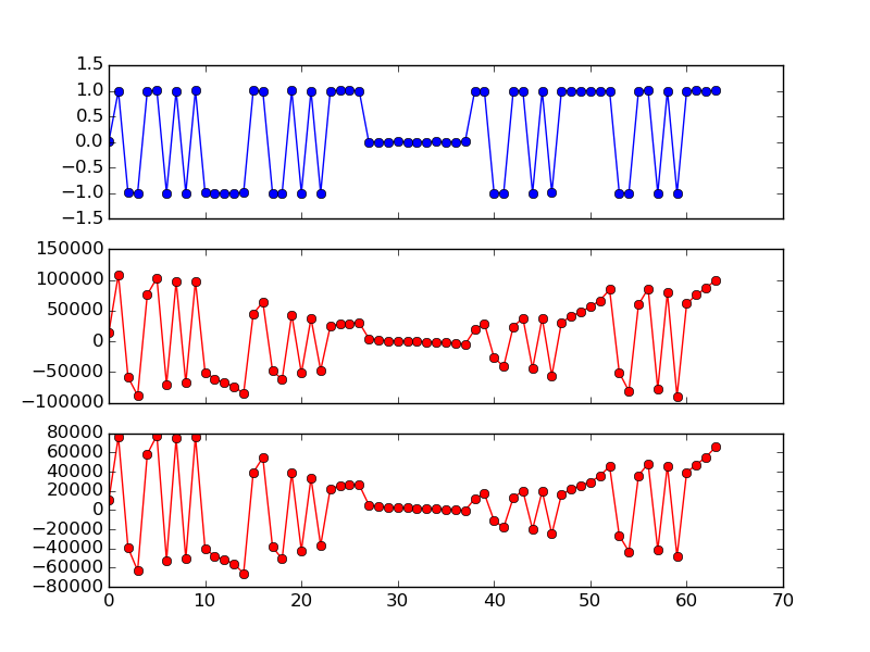
Fig. 14 FFT of the Perfect and Two Actual LTS
To plot Fig. 14:
lts1 = samples[11+160:][32:32+64]
lts2 = samples[11+160:][32+64:32+128]
fig, ax = plt.subplots(nrows=3, ncols=1, sharex=True);
ax[0].plot([c.real for c in np.fft.fft(lts)], '-bo');
ax[1].plot([c.real for c in np.fft.fft(lts1)], '-ro');
ax[2].plot([c.real for c in np.fft.ff t(lts2)], '-ro');
plt.show()
Fig. 14 shows the FFT of the perfect LTS and the two actual LTSs in the samples. We can see that each sub-carrier exhibits different magnitude gain. In fact, they also have different phase drift. The combined effect of magnitude gain and phase drift (known as channel gain) can clearly be seen in the I/Q plane shown in Fig. 15.
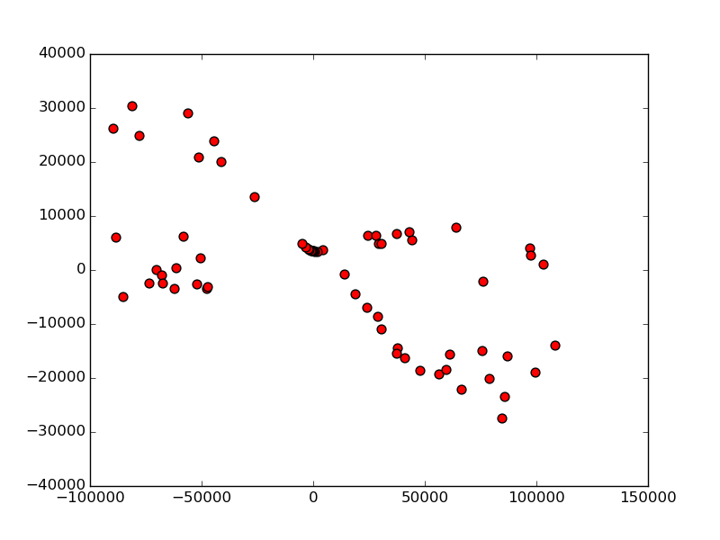
Fig. 15 FFT in I/Q Plane of The Actual LTS
To map the FFT point to constellation points, we need to compensate for the channel gain. This can be achieved by normalize the data OFDM symbols using the LTS. In particular, the mean of the two LTS is used as channel gain (\(H\)):
where \(L[i]\) is the sign of the LTS sequence:
And the FFT output at sub-carrier \(i\) is normalized as:
where \(X[i]\) is the FFT output at sub-carrier \(i\).
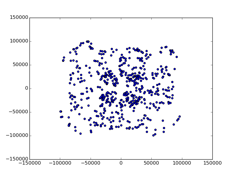
Fig. 16 FFT Without Normalization
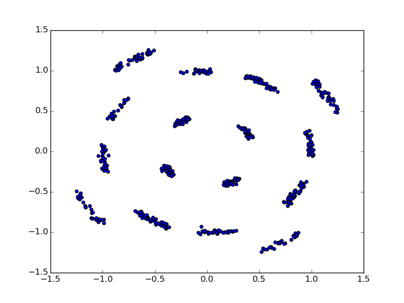
Fig. 17 FFT With Normalization
Fig. 16 and Fig. 17 shows the FFT before and after normalization using channel gain.
Residual Frequency Offset Correction
We can see from Fig. 17 that the FFT output is tilted slightly. This is caused by residual frequency offset that was not compensated during the coarse CFO correction step.
This residual CFO can be corrected either by Fine CFO Correction, or/and by the
pilot sub-carriers. Ideally we want to do both, but since the fine CFO is
usually beyond the resolution of the phase look up table, we skip it in the
sync_long.v module and only rely on the pilot sub-carriers.
Regardless of the data sub-carrier modulation, the four pilot sub-carriers (-21, -7, 7, 21) always contains BPSK modulated pseudo-random binary sequence.
The polarity of the pilot sub-carriers varies symbol to symbol. For 802.11a/g, the pilot pattern is:
And the pilot sub-carriers at OFDM symbol \(n\) (starting at 0 from the first symbol after the long preamble) is then:
For 802.11n at 20MHz bandwidth with single spatial stream, the n’th pilot sub-carriers are:
And:
In other words, the pilot sub-carries of the first few symbols are:
For other configurations (e.g., spatial stream, bandwidth), the pilot
sub-carrier pattern can be found in Section 20.3.11.10 in
802.11-2012 std.
The residual phase offset at symbol \(n\) can then be estimated as:
Combine this phase offset and the previous channel gain correction together, the adjustment to symbol \(n\) is:
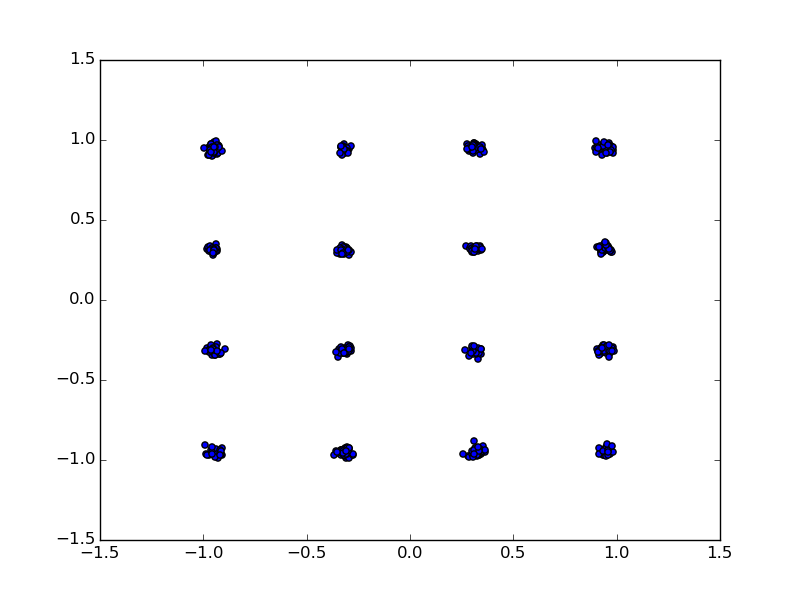
Fig. 18 Residual CFO Correction Using Pilot Sub-Carriers
Fig. 18 shows the effect of correcting the residual CFO using pilot sub-carriers. Each sub-carrier can then be mapped to constellation points easily.
In OpenOFDM, the above tasks are implemented by the equalizer.v module.
It first stores the first LTS, and then calculates the mean of the two LTS and
store it as channel gain.
For each incoming OFDM symbol, it first obtains the polarity of the pilot sub-carriers in current symbol, then calculates the residual CFO using the pilot sub-carriers and also performs the channel gain correction.